We have already used aggregate analysis several times in this course. For example, when analyzing the BFS and DFS procedures, instead of trying to figure out how many times their inner loops
for each v ∈ G.Adj[u]
execute (which depends on the degree of the vertex being processed), we realized that no matter how the edges are distributed, there are at most |E| edges, so in aggregate across all calls the loops will execute |E| times.
But that analysis concerned itself only with the complexity of a single operation. In practice a given data structure will have associated with it several operations, and they may be applied many times with varying frequency.
Sometimes a given operation is designed to pay a larger cost than would otherwise be necessary to enable other operations to be lower cost.
Example: Red-black tree insertion. We pay a greater cost for balancing so that future searches will remain O(lg n).
Another example: Java Hashtable.
It is "fairer" to average the cost of the more expensive operations across the entire mix of operations, as all operations benefit from this cost.
Here, "average" means average cost in the worst case (no probability is involved, which greatly simplifies the analysis).
We will look at three methods. The notes below use Stacks with Multipop to illustrate the methods. See the text for binary counter examples.
(We have already seen examples of aggregate analysis throughout the semseter. We will see examples of amortized analysis later in the semester.)
We already have the stack operations:
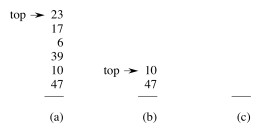
Suppose we add a Multipop (this is a generalization of ClearStack, which empties the stack):


The example shows a Multipop(S,4) followed by another where k ≥ 2.
Running time of Multipop:
What is the worst case of a sequence of n Push, Pop and Multipop operations?
Using our existing methods of analysis we can identify a loose bound over n operations:
Can you see a flaw in this reasoning?
We can tighten this loose bound by aggregating the analysis over all n operations:
This analysis shows O(1) per operation on average in a sequence of n operations without using any probabilities of operations.
See the CLRS text for an example of aggregate analysis of binary counting. An example of aggregate analysis of dynamic tables is at the end of these notes.
Some of our previous analyses with indicator random variables have been a form of aggregate analysis, specifically our analysis of the expected number of inversions in sorting, Topic 5, and our analysis of Depth-First Search, Topic 14.
Aggregate analysis treats all operations equally. The next two methods let us give different operations different costs, so are more flexible.
The amortized cost is the amount we charge each operation, which may be different from the operation actually costs.
This differs from aggregate analysis:
When an operation is overcharged (amortized cost > actual cost), the difference is associated with specific objects in the data structure as credit.
We use this credit to pay for operations whose actual cost > amortized cost.
The credit must never be negative. Otherwise the amortized cost may not be an upper bound on actual cost for some sequences.
Let
Require ∑i=1,n ĉi ≥ ∑i=1,n ci for all sequences of n operations. That is, the difference between these sums is always ≥ 0: we never owe anyone anything, and ĉ will provide an upper bound on the actual cost for all sequences.
Whenever we Push an object (at actual cost of 1 cyberdollar), we potentially have to pay CY$1 in the future to Pop it, whether directly or in Multipop.
To make sure we have enough money to pay for the Pops, we charge Push CY$2.
Since each object has CY$1 credit, the credit can never go negative.

The total amortized cost ĉ = ∑i=1,n ĉi for any sequence of n operations is an upper bound on the total actual cost c = ∑i=1,n ci for that sequence. This is clearly true in the case of PUSH operations where the amortized cost $2 is greater than the actual cost $1. It is true for the other operations because they can only incur an actual cost of $1 per item when operating on items in the stack, and there will be $1 credit associated with each item.
Since ĉ = O(n), also c = O(n).
Note: we don't actually store cyberdollars in any data structures. This is just a metaphor to enable us to compute an amortized upper bound on costs.
Does it seem strange that we charge Pop and Multipop 0 when we know they cost something?
Instead of credit associated with objects in the data structure, this method uses the metaphor of potential associated with the entire data structure.
(I like to think of this as potential energy, but the text continues to use the monetary metaphor.)
This is the most flexible of the amortized analysis methods, as it does not require maintaining an object-to-credit correspondence.
Let
The Potential Function Φ: Di → ℜ maps states to real numbers (the potential). We say that Φ(Di) is the potential associated with the data structure in state Di.
We define the amortized cost ĉi to be the actual cost ci plus the change in potential due to the ith operation:
ĉi = ci + Φ(Di) − Φ(Di-1)
The total amortized cost across n operations is:
∑i=1,n ĉi = ∑i=1,n(ci + Φ(Di) - Φ(Di-1)) = (∑i=1,n ci) + (Φ(Dn) - Φ(D0))
The last step is taken because the middle expression involves a telescoping sum: every term other than Dn and D0 is added once and subtracted once.
If we require that Φ(Di) ≥ Φ(D0) for all i then the amortized cost will always be an upper bound on the actual cost no matter which ith step we are on.
This is usually accomplished by defining Φ(D0) = 0 and then showing that Φ(Di) ≥ 0 for all i. (Note that this is a constraint on Φ, not on ĉ. ĉ can go negative as long as Φ(Di) never does.)
Define Φ(Di) = number of objects in the stack.
Then Φ(D0) = 0 and Φ(Di) ≥ 0 for all i, since there are never less than 0 objects on the stack.
Charge as follows (recalling that ĉi = ci + Φ(Di) - Φ(Di-1), the "actual cost" column is ci, and the 'ΔΦ" column computes the difference Φ(Di) - Φ(Di-1)):

Since we charge 2 for each Push and there are O(n) Pushes in the worst case, the amortized cost of a sequence of n operations is O(n).
There is often a tradeoff between time and space, for example, with hash tables. Bigger tables give faster access but take more space.
Dynamic tables, like the Java Hashtable, grow dynamically as needed to keep the load factor reasonable.
Reallocation of a table and copying of all elements from the old to the new table is expensive!
But this cost is amortized over all the table access costs in a manner analogous to the stack example: We arrange matters such that table-filling operations build up sufficient credit before we pay the large cost of copying the table; so the latter cost is averaged over many operations.
Load factor α = num/size, where num = # items stored and size = the allocated size of the table.
For the boundary condition of size = num = 0, we will define α = 1.
We never allow α > 1 (no chaining).
We'll assume the following about our tables. (See Exercises 17.4-1 and 17.4-3 concerning different assumptions.):
When the table becomes full, we double its size and reinsert all existing items. This guarantees that α ≥ 1/2, so we are not wasting a lot of space.
  Table-Insert (T,x)
    1  if T.size == 0
    2      allocate T.table with 1 slot
    3      T.size = 1
    4  if T.num == T.size
    5      allocate newTable with 2*T.size slots
    6      insert all items in T.table into newTable
    7      free T.table
    8      T.table = newTable
    9      T.size = 2*T.size
   10  insert x into T.table
   11  T.num = T.num + 1
Each elementary insertion insert x into T.table has unit actual cost. Initially T.num = T.size = 0.
Charge 1 per elementary insertion (including copying items into a new table). Count only these insertions, since all other costs are constant per call.
ci = actual cost of ith operation (number of items inserted).
A sloppy analysis: In a sequence of n operations where any operation can be O(n), the sequence of n operations is O(n2).
This is "correct", but inprecise: we rarely expand the table! A more precise account of ci is based on the fact that if we start with a table of size 1 and double its size every time we expand it, we do the expansions when the number of items in the table is a power of 2:

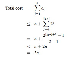
Then we can sum the total cost of all ci for a sequence of n operations:


Explanation of steps:
Therefore, the amortized cost per operation = 3: we are only paying a small constant price for the expanding table.
We charge CY$3 for each insertion into the table, i.e., the amortized cost of the i-th insertion as ĉi = 3. The actual cost of the i-th insertion is as before:

We must show that we never run out of credit. It's equivalent to proving the following Lemma.
Lemma: For any sequences of n insertions ∑i=1,n ĉi ≥ ∑i=1,n ci.
Proof: By using the same equation as above, we know that for any n: ∑i=1,n ci ≤ 3n. By the definition of ĉ, we know that: ∑i=1,n ĉi = 3n. The lemma follows. ∎
That's it!
In case it helps to understand why this works:
We charge CY$3 for inserting some item x into the table. Obviously, we are overcharging for each simple insertion which costs only CY$1. However, the overcharging will provide enough credit to pay for future copying of items when the table becomes full:
But the table might need to be expanded more than once after x is inserted, so x might need to be copied more than once. Who will pay for future copying of x? That's where the third CY$1 comes in:
Let's see why CY$3 is enough to cover all possible future exansions and copying associated with them.
The text also provides the potential analysis of table expansion.
This analysis assumed that the table never shrinks. See section 17.4 for an analysis using the potential method that covers shrinking tables.
Here are some other algorithms for which amortized analysis is useful:
An amortized analysis of Red-Black Tree restructuring (Problem 17-4 of CLRS) improves upon our analysis earlier in the semester:
Amortized analysis will be used in analyses of