Multithreading is a crucial topic for modern computing. Parallel machines are getting cheaper and in fact are now ubiquitous ...
Our emphasis here will be parallel algorithms, that is, multithreading a single algorithm so that some of its instructions may be executed simultaneously. Parallelism can also be applied to scheduling and managing multiple algorithms, each running concurrently in their own thread and possibly sharing resources, as studied in courses on operating systems and concurrent and high performance computing.
Static threading provides the programmer with an abstraction of virtual processors that are managed explicitly. It's "static" because the programmer must specify in advance how many processors to use at each point. This can be difficult and inflexible with respect to evolving conditions.
Rather than managing threads explicitly, our model is dynamic multithreading in which programmers specify opportunities for parallelism, and a concurrency platform manages the decisions of mapping these opportunities to actual static threads.
We will use three keywords in our pseudocode, reflecting current parallel-computing practice:
These keywords specify opportunities for parallelism without affecting whether (or not) the corresponding sequential program obtained by removing them is correct. In other words, if we ignore the parallel keywords the program can be analyzed as a single threaded program. We exploit this in analysis.
The parallel and spawn keywords do not force parallelism: they just says that it is permissible. This is logical parallelism. A scheduler will make the decision concerning allocation to processors. We return to the question of scheduling at the end of this document, after approriate concepts have been introduced.
However, if parallelism is used, sync must be respected. For safety, there is an implicit sync at the end of every procedure.
For illustration, we take a really slow algorithm and make it parallel. (There are much better ways to compute Fibonacci numbers using dynamic programming; this is just for illustration.) Here is the definition of Fibonacci numbers:
F0 = 0.
F1 = 1.
Fi = Fi-1 + Fi-2, for i ≥ 2.
Here is a recursive non-parallel algorithm for computing Fibonacci numbers modeled on the above definition, along with its recursion tree:
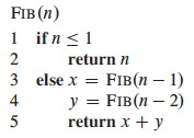
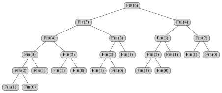
Fib has recurrence relation T(n) = T(n − 1) + T(n − 2) + Θ(1), which has the solution T(n) = Θ(Fn) (see the text for substitution method proof). This grows exponentially in n, so it's not very efficient. (A straightforward iterative algorithm is much better.)
Noticing that the recursive calls operate independently of each other, let's see what improvement we can get by computing the two recursive calls in parallel. This will illustrate the concurrency keywords and also be an example for analysis:
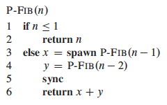
Notice that without the parallel keywords it is the same as the serial program above.
We will return to this example when we analyze multithreading.
First we need a formal model to describe parallel computations.
We will model a multithreaded computation as a computation DAG (directed acyclic graph) G = (V, E):
We assume an ideal parallel computer with sequentially consistent memory, meaning it behaves as if the instructions were executed sequentially in some full ordering consistent with orderings within each thread (i.e., consistent with the partial ordering of the computation DAG).
The model can be visualized as exemplified below for the computation DAG for P-Fib(4):

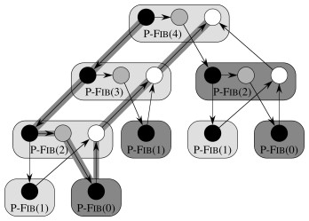
Vertices (strands) are visualized as circles in the figure.
Edges are categorized and visualized as follows:
We write TP to indicate the running time of an algorithm on P processors. Then we define these measures and laws:
T1 = the total time to execute an algorithm on one processor. This is called work in analogy to work in physics: the total amount of computational work that gets done.
An ideal parallel computer with P processors can do at most P units of work in one time step. So, in TP time it can do at most P⋅TP work. Since the total work is T1, P⋅TP ≥ T1, or dividing by P we get the work law:
TP ≥ T1 / P
The work law can be read as saying that the speedup for P processors can be no better than the time with one processor divided by P. That is,
parallelism on P processors at best gives constant speedup where the constant is 1/P.
Parallelism will not change the asymptotic class of an algorithm: it's not a substitute for careful design of asymptotically fast algorithms.
The span of a multithreaded computation is the longest time to execute the strands along any path in the computation DAG. If each strand (represented by vertices) takes a unit of time, then this will be the number of vertices on the longest path in the DAG, which we call the critical path. If strands take different amounts of time then the critical path will be the path with the greatest cost, summing the costs associated with the vertices.

(Readers in our classes may recall the class excercise on finding the shortest time you can complete a set of interdependent jobs by finding the longest path in the job DAG: the concept here is similar.)
We can also define span as T∞ = the total time to execute an algorithm on an infinite number of processors — or, more practically speaking, on just as many processors as are needed to allow parallelism wherever it is possible. It is the fastest we can possibly expect — an Ω bound -- because no matter how many processors you have, the algorithm must take this long.
The critical path in our P-Fib example is represented by the shaded edges in the figure. Notice that span is not simply the costs on the path from the root to the leaves of the recursion tree: Once the recursion has hit the base case the execution still needs to proceed as the recursion unwinds.
The span law states that a P-processor ideal parallel computer cannot run faster than one with an infinite number of processors:
TP ≥ T∞
This is because at some point the span will limit the speedup possible: No matter how many processors you have, you still must do these strands in sequence, taking the time they require.
Exercise: If we count each vertex as one unit of work, what is the work and span of the computation DAG for P-Fib shown?
The ratio T1 / TP defines how much speedup you get with P processors as compared to one.
By the work law,
TP ≥ T1 / P, so T1 / TP ≤ P:
one cannot have any more speedup than the number of processors.
This is important enough to repeat: parallelism provides only constant time improvements (the constant being the number of processors) to any algorithm! Parallelism cannot move an algorithm from a higher to lower complexity class (e.g., exponential to polynomial, or quadratic to linear). Parallelism is not a silver bullet: good algorithm design and analysis is still needed.
When the speedup T1 / TP = Θ(P) we have linear speedup: the speedup is linear in the number of processors.
When T1 / TP = P we have perfect linear speedup: we got the maximum amount of speedup possible from each processor.
The ratio T1 / T∞ of the work to the span gives the (potential) parallelism of the computation. It can be interpreted in three ways:
This latter way of looking at T1 / T∞ leads to the concept of parallel slackness:
(T1 / T∞) / P = T1 / (P⋅T∞),
the factor by which the parallelism of the computation exceeds the number of processors in the machine. We have three cases:
Exercise: What is the parallelism of the computation DAG for P-Fib shown previously? What does this parallelism say about the prospects for speedup at *this* n? What happens to work and span as n grows?
Analyzing work is simple: ignore the parallel constructs and analyze the serial algorithm.
For example, we already noted previously that the work of P-Fib(n) is
T(n) = T(n − 1) + T(n − 2)+ Θ(1),
which has the solution T(n) = Θ(Fn), the work of P-Fib(n).
Analyzing span requires a different approach. (I hope you did the exercises above: they will make you appreciate the following all the more.)
If a set of subcomputations (or the vertices representing them) are in series, the span is the sum of the spans of the subcomputations. This is like normal sequential analysis (as was just exemplified above with the sum T(n − 1) + T(n − 2)).
If a set of subcomputations (or the vertices representing them) are in parallel, the span is the maximum of the spans of the computations. This is where analysis of multithreaded algorithms differs.

Returning to our example, the span of the parallel recursive calls of P-Fib(n) is computed by taking the max rather than the sum:
T∞ (n) = max(T∞(n−1), T∞ (n−2)) + Θ(1)
= T∞(n−1) + Θ(1).
The recurrence T∞ (n) = T∞(n−1) + Θ(1) has solution Θ(n). So the span of P-Fib(n) is Θ(n).
We can now compute the parallelism of P-Fib(n) in general (not just the specific case of n=4 that we computed earlier) by dividing its work Θ(Fn) by its span Θ(n):
T1(n) / T∞ = Θ(Fn) / Θ(n) = Θ(Fn/n)This grows dramatically, as Fn grows much faster than n.
For any given number of processors P, there is considerable parallel slackness Θ(Fn/n)/P. For any P above some n there is likely to be something for additional processors to do. Thus there is potential for near perfect linear speedup as n grows.
Of course in this example it's because we chose an inefficent way to compute Fibonacci numbers, but this was only for illustration. These ideas apply to other well designed algorithms.
So far we have used spawn, but not the parallel keyword, which is used with loop constructs such as for. Here is an example.
Suppose we want to multiply an n x n matrix A = (aij) by an n-vector x = (xj). This yields an n-vector y = (yi) where:

The following algorithm does this in parallel:
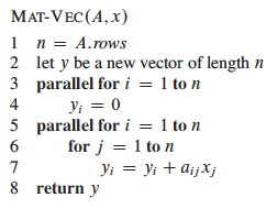
The parallel for keywords indicate that each iteration of the loop can be executed concurrently. (Notice that the inner for loop is not parallel; a possible point of improvement to be discussed.)
It is not realistic to think that all n subcomputations in these loops (lines 3 and 5) can be spawned simultaneously with no extra work. (For some operations on some hardware up to a constant n this may be possible; e.g., hardware designed for matrix operations; but we are concerned with the general case.) How might this parallel spawning be done, and how does this affect the analysis?
Parallel for spawning can be accomplished by a compiler with a divide and conquer approach, itself implemented with parallelism!
Consider how to implement parallelism in lines 5-7 of Mat-Vec above. The concurrency platform compiler can arrange for the procedure shown below to be called instead, Mat-Vec-Main-Loop(A, x, y, n, 1, n). Lines 2 and 3 below are the lines originally within the loop.
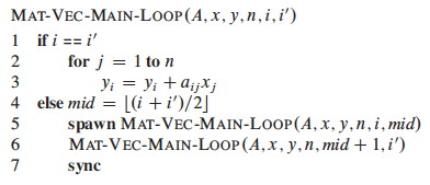
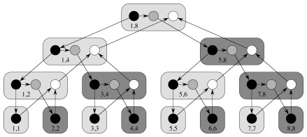
The computation DAG is also shown. It appears that a lot of work is being done to spawn the n leaf node computations, but the increase is not asymptotically significant.
The work of Mat-Vec is T1(n) = Θ(n2) due to the nested loops in 5-7.
Since the computation DAG is a full binary tree, the number of internal nodes is 1 fewer than the n leaf nodes (Topic 8), so this extra work is Θ(n).
Each leaf node corresponds to one iteration of loop, and the extra work of recursive spawning can be amortized across the work of the iterations, so that it contributes only constant work.
Concurrency platforms sometimes coarsen the recursion tree by executing several iterations in each leaf, reducing the amount of recursive spawning.
The span is increased by Θ(lg n) due to the addition of the recursion tree for Mat-Vec-Main-Loop, which is of height Θ(lg n). In some cases (such as this one), this increase is washed out by other dominating factors (e.g., the span in this example is dominated by the nested loops).
Continuing with our example, the span is Θ(n) because even with full utilization of parallelism the inner for loop still requires Θ(n). Since the work is Θ(n2) the parallelism is Θ(n2)/Θ(n) = Θ(n). Can we improve on this?
Perhaps we could make the inner for loop parallel as well? Compare the original to the revised version Mat-Vec':

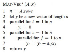
Would it work? We need to introduce a new concept ...
Deterministic algorithms do the same thing on the same input; while nondeterministic algorithms may give different results on different runs.
The above Mat-Vec' algorithm is subject to a potential problem called a determinancy race: when the outcome of a computation could be nondeterministic (unpredictable). In general, this can only happen when two logically parallel computations access the same memory and one performs a write.
Determinancy races are hard to detect with empirical testing: many execution sequences would give correct results. This kind of software bug is consequential: Race condition bugs caused the Therac-25 radiation machine to overdose patients, killing three; and caused the North American Blackout of 2003.
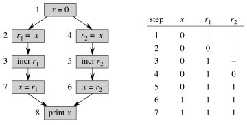
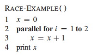
For example, the code shown below might output 1 or 2 depending on the order in which access to x is interleaved by the two threads:
The value of x must first be read into a register r before it is operated on. In this case, there are two registers. It is incremented in the register and then written back out to memory. The table indicates one possible computation sequence that gives the unexpected result.
After you understand that simple example, let's look at our (renamed) matrix-vector example again:
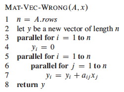
Exercise: Do you see how yi might be updated differently depending on the order in which parallel invocations of line 7 (including access to current value of yi and writing new ones) are executed? Keep in mind that race conditions can only happen when two logically parallel computations access the same memory and one performs a write.
Here is an algorithm for multithreaded matrix multiplication, based on the T1(n) = Θ(n3) algorithm:
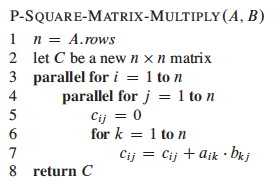
Exercise: How does this procedure compare to MAT-VEC-WRONG? Both of them have nested parallel for loops: Is P-SQUARE-MATRIX-MULTIPLY also subject to a race condition? Why or why not?
The span of this algorithm is T∞(n) = Θ(n), due to the path for spawning the outer and inner parallel loop executions and then the n executions of the innermost for loop. So the parallelism is T1(n) / T∞(n) = Θ(n3) / Θ(n) = Θ(n2)
Exercise: Could we get the span down to Θ(1) if we parallelized the inner for with parallel for? You should be able to answer this based on the previous exercise.
Here is a parallel version of the divide and conquer algorithm from Chapter 4 of CLRS (not in these web notes):
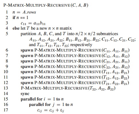
See the text for analysis, which concludes that while the work is still Θ(n3), the span is reduced to Θ(lg2n). Thus, while the work is the same as the basic algorithm the parallelism is Θ(n3) / Θ(lg2n), which makes good use of parallel resources.
Divide and conquer algorithms are good candidates for parallelism, because they break the problem into independent subproblems that can be solved separately. We look briefly at merge sort.
The dividing is in the main procedure MERGE-SORT, and we can parallelize it by spawning the first recursive call:
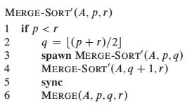
MERGE remains a serial algorithm, so its work and span are Θ(n) as before.
The recurrence for the work MS'1(n) of MERGE-SORT' is the same as the serial version:

The recurrence for the span MS'∞(n) of MERGE-SORT' is based on the fact that the recursive calls run in parallel, so there is only one n/2 term (they are the same, so min takes either):

The parallelism is thus MS'1(n) / MS'∞(n) = Θ(n lg n / n) = Θ(lg n).
This is low parallelism, meaning that even for large input we would not benefit from having hundreds of processors. How about speeding up the serial MERGE?
MERGE takes two sorted lists and steps through them together to construct a single sorted list. This seems intrinsically serial, but there is a clever way to make it parallel.
A divide-and-conquer strategy can rely on the fact that the lists are sorted to break the lists into four lists, two of which will be merged to form the head of the final list and the other two merged to form the tail.
To find the four lists for which this works, we
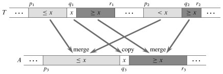
The text presents the BINARY-SEARCH pseudocode and analysis of Θ(lg n) worst case; this should be review for you. It then assembles these ideas into a parallel merge procedure that merges into a second array Z at location p3 (r3 is not provided as it can be computed from the other parameters):
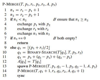
My main purpose in showing this to you is to see that even apparently serial algorithms sometimes have a parallel alternative, so we won't get into details, but here is an outline of the analysis:
The span of P-MERGE is the maximum span of a parallel recursive call. Notice that although we divide the first list in half, it could turn out that x's insertion point q2 is at the beginning or end of the second list. Thus (informally), the maximum recursive span is 3n/4 (as at best we have "chopped off" 1/4 of the first list).
The text derives the recurrence shown below; it does not meet the Master Theorem, so an approach from a prior exercise is used to solve it:

Given 1/4 ≤ α ≤ 3/4 for the unknown dividing of the second array, the work recurrence turns out to be:

With some more work, PM1(n) = Θ(n) is derived. Thus the parallelism is Θ(n / lg2n)
Some adjustment to the MERGE-SORT' code is needed to use this P-MERGE; see the text. Further analysis shows that the work for the new sort, P-MERGE-SORT, is PMS1(n lg n) = Θ(n), and the span PMS∞(n) = Θ(lg3n). This gives parallelism of Θ(n / lg2n), which is much better than Θ(lg n) in terms of the potential use of additional processors as n grows.
The chapter ends with a comment on coarsening the parallelism by using an ordinary serial sort once the lists get small. One might consider whether P-MERGE-SORT is still a stable sort, and choose the serial sort to retain this property if it is desirable.
At the beginning, we noted that we rely on a concurrency platform to determine how to allocate potentially parallel threads of computation to available processors. This is the scheduling problem. Scheduling parallel computations is a complex problem, and sophisticated schedulers have been designed that are beyond what we can discuss here.
Centralized schedulers are those that have information on the global state of computation, but must make decisions in real time rather than in batch. A simple approach to centralized scheduling is a greedy scheduler, which assigns as many strands to available processors as possible at any given time step. The CLRS texts proves a theorem concerning the performance of a greedy scheduler, with interesting corollaries:
Theorem: On an ideal parallel computer with P processors, a greedy scheduler executes a multithreaded computation with work T1 and span T∞ in time TP ≤ T1 + T∞.
Corollary: The running time TP of any multithreaded computation scheduled by a greedy scheduler on an ideal parallel computer with P processors is within a factor of 2 of optimal.
Corollary: As slackness grows a greedy scheduler achieves near-perfect linear speedup on any multithreaded computation.
The proofs are not difficult to understand: see the text if you are interested. I think we have said enough here to introduce the concepts of multithreading.
Professor Henri Casanova does research on scheduling, and Professor Nodari Sitchinava does research on parallel algorithms. They would be happy to talk to interested students.